
在未来几年,深度学习会改变前端开发,它会提高基于原型的开发速度,降低开发软件的成本。
随着 Tony Beltramelli 发起的 pix2code 和 Airbnb 发起的 sketch2code 项目的发展,这一领域正在飞速发展。
目前,前端开发智能化的最大阻碍是计算能力。不管怎样,我们可以使用当下流行的深度学习算法,以及现成的训练数据,来探索一下机器开发前端。
1)把设计图片输入给训练过的神经网络

2)神经网络把图片转换成 HTML 代码
3)渲染输出

我们将会分三步构建神经网络。
首先,我们将会实现一个基础功能版本熟悉一下流程。第二个是 HTML 版本,会将所有的操作自动化,这里会介绍神经网络层。在最终的 Booststrap 版本里,我们将创建一个通用的 LSTM 层模型。
代码托管在 GitHub 和 FloyHub Jupyter 的 notebooks 上。所有的 FloydHub notebooks 在 floydhub 目录下,本地文件在 local 目录下。
模型基于 Beltramelli 的 pix2code paper 以及 Jason Brownlee 的图片识别教程。代码是 Python 和 Keras 写的,Keras 是一个基于 TensorFlow 的框架。
如果你是深度学习的新手,建议你从 Python 、backpropagation 和卷积神经网络开始入门。我在 FloyHub 的三篇早期博客(英文)可以作为参考:
核心概念
让我们来看一下我们的目标。我们想要构建一个神经网络,它可以根据网页截图生成相应的 HTML/CSS 代码。
通过和截图匹配的 HTML 代码来训练神经网络。
机器通过把 HTML 代码标签和相应的图片对比来学习。它分析截图以找到合适的 HTML 标签。
这里是 Google Sheet 上的一组简单的训练数据例子。
创建逐字预测的模型是普遍做法。当然还有其它的方法,为了便于理解,我们在教程里采用普遍做法。
注意每次预测都是读取同一个图片。所以如果预测 20 个单词,会读取 20 次原型图。目前为止,不用太纠结神经网络是如何工作的,了解神经网络的输入和输出就好了。

先从上一个标签开始处理。训练机器来识别句子 “I can code” 。当输入 “I”,它会预测出 “can”。下一次输入变成 “I can” 然后预测出 “code”。输入一个单词就能预测出下一个单词。

神经网络从数据里寻找特征,然后通过特征建立输入和输出的联系。它会创建画像来了解每一个截图是什么,然后预测 HTML 语句。从而构建出知识体系来预测标签。
把训练好的模型应用于真实世界,和模型训练的原理是相同的。文字也是根据截图逐个生成。区别是它根据已经学习过的标签来预测代码,而不是给定相应的 HTML 代码来学习。接着,预测下一个代码标签。预测从 “开始标签” 预测,在 “结束标签” 或者达到最大限制截止。这里是在 Google Sheet 上的另一个例子。

“hello world” 版本
让我们先来构建一个 “hello world” 版本。先让神经网络学习一个显示 “Hello World” 的网站截图,教他生成相应标签。
首先,神经网络把设计原型图转换为像素值列表。值范围是 0 - 255,包含红蓝绿三个通道。

这里使用了 one hot encoding 把标签转换成神经网络可以理解的方式。例如,句子 “I can code” 可以转换成下面的样子。

在上面的图片里,还包含了开始和结束标记。这些标记代表了机器什么时候开始识别什么时候终止识别。
我们使用句子作为数据输入,从第一个单词开始,接着一个单词一个单词的添加。输出数据也是单词。
句子的逻辑和单词是一样的,也同样需要输入长度。句子受最大句子长度约束,而不是受最低词汇量限制。如果句子长度比最大长度短,会使用 0 字符填充。

如你所见,单词从右到左打印。每轮训练单词的位置都不固定。这样模型就可以学习句子而不是简单记住每个单词的位置。
在下面的图片里有四个预测。每一行是一个预测。左边的图片表示三个颜色通道: 红、绿、蓝,以及当前的单词。括号外面代表每次的预测,红色的方块代表结束。

green blocks = start tokens | red block = end token
#Length of longest sentence
max_caption_len = 3
#Size of vocabulary
vocab_size = 3
# Load one screenshot for each word and turn them into digits
images = []
for i in range(2):
    images.append(img_to_array(load_img('screenshot.jpg', target_size=(224, 224))))
images = np.array(images, dtype=float)
# Preprocess input for the VGG16 model
images = preprocess_input(images)
#Turn start tokens into one-hot encoding
html_input = np.array(
            [[[0., 0., 0.], #start
             [0., 0., 0.],
             [1., 0., 0.]],
             [[0., 0., 0.], #start <HTML>Hello World!</HTML>
             [1., 0., 0.],
             [0., 1., 0.]]])
#Turn next word into one-hot encoding
next_words = np.array(
            [[0., 1., 0.], # <HTML>Hello World!</HTML>
             [0., 0., 1.]]) # end
# Load the VGG16 model trained on imagenet and output the classification feature
VGG = VGG16(weights='imagenet', include_top=True)
# Extract the features from the image
features = VGG.predict(images)
#Load the feature to the network, apply a dense layer, and repeat the vector
vgg_feature = Input(shape=(1000,))
vgg_feature_dense = Dense(5)(vgg_feature)
vgg_feature_repeat = RepeatVector(max_caption_len)(vgg_feature_dense)
# Extract information from the input seqence
language_input = Input(shape=(vocab_size, vocab_size))
language_model = LSTM(5, return_sequences=True)(language_input)
# Concatenate the information from the image and the input
decoder = concatenate([vgg_feature_repeat, language_model])
# Extract information from the concatenated output
decoder = LSTM(5, return_sequences=False)(decoder)
# Predict which word comes next
decoder_output = Dense(vocab_size, activation='softmax')(decoder)
# Compile and run the neural network
model = Model(inputs=[vgg_feature, language_input], outputs=decoder_output)
model.compile(loss='categorical_crossentropy', optimizer='rmsprop')
# Train the neural network
model.fit([features, html_input], next_words, batch_size=2, shuffle=False, epochs=1000)
在 hello world 版本里,用到了 3 个 tokens: start、<HTML><center><H1>Hello World!</H1></center></HTML> 和 end。token 可以是任何东西。可以是字符、单词或者句子。字符版本需要较少的词汇量,但是受限于神经网络。单词版本则性更优。
下面是做出的预测:
# Create an empty sentence and insert the start token
sentence = np.zeros((1, 3, 3)) # [[0,0,0], [0,0,0], [0,0,0]]
start_token = [1., 0., 0.] # start
sentence[0][2] = start_token # place start in empty sentence

# Making the first prediction with the start token
second_word = model.predict([np.array([features[1]]), sentence])

# Put the second word in the sentence and make the final prediction
sentence[0][1] = start_token
sentence[0][2] = np.round(second_word)
third_word = model.predict([np.array([features[1]]), sentence])

# Place the start token and our two predictions in the sentence
sentence[0][0] = start_token
sentence[0][1] = np.round(second_word)
sentence[0][2] = np.round(third_word)

# Transform our one-hot predictions into the final tokens
vocabulary = ["start", "<HTML><center><H1>Hello World!</H1></center></HTML>", "end"]
for i in sentence[0]:
print(vocabulary[np.argmax(i)], end=' ')
输出
- 10 epochs:
start start start - 100 epochs:
start <HTML><center><H1>Hello World!</H1></center></HTML> <HTML><center><H1>Hello World!</h1></center></HTML> - 300 epochs:
start <HTML><center><H1>Hello World!</H1></center></HTML> end
我犯的错误
- 构建前先收集数据。 在这个项目初期,我设法获取了 Geocities 托管网站的一个旧的副本。上面有三千八百万个网站。由于过于盲目,我忽略了分析 10 万词汇量所需的巨大工作。
- 处理 TB 级别的数据需要一个好的设备以及很大的耐心。 在 mac 运行力不从心后,我开始使用更强大的远程服务器。租用的 8 核 CPU 1G 带宽让我有了一个像样的调试环境。
- 在我熟悉数据输入输出之前一切都没用。 输入 X,是一个截图以及前一个标签代码。输出,Y,是下一个标签代码。当我理清这些时,事情变得简单多了。切换不同的架构也变得很方便。
- 当心未知世界。 由于这个项目涉及到深度学习的很多领域,在学习过程中我在好多不必要的地方浪费了大量时间。我花了一周时间从零开始学习 RNNs,研究了一段时间嵌入向量空间,又了解了各种非主流实现。
- 机器图片转代码是一种图片识别模型。 当我了解到这一点时,我仍然忽略了很多图片识别资料,因为它们太枯燥了。一旦我意识到这一点,我的进步飞快。
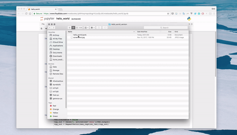
在 FloydHub 上运行代码
FloydHub 是一个深度学习训练平台。我第一次接触深度学习的时候就开始用它,现在我用它来处理机器学习并记录我的学习过程。你可以点击下面的按钮在 30s 内快速上手:

这个链接在 FloydHub 上打开了一个工作空间,里面包含了 Bootstrap 版本所使用的环境和数据集。以及测试用的训练好的模型。
或者你可以通过以下这两步手动安装: 2 分钟安装 、5 分钟上手教程。
克隆仓库
git clone https://github.com/emilwallner/Screenshot-to-code-in-Keras.git
登录并初始化 FloydHub 命令行工具
cd Screenshot-to-code-in-Keras
floyd login
floyd init s2c
在FloydHub 云 GPU 机器上运行 Jupyter 笔记本
floyd run --gpu --env tensorflow-1.4 --data emilwallner/datasets/imagetocode/2:data --mode jupyter
所有的 notebooks 都在 FloydHub 路径下。local 代表本地。一旦运行,你可以在这里找到第一个 notebook:floydub/Helloworld/helloworld.ipynd。
如果你想要更详细的介绍,这里有一篇我早期的文章。
HTML 版本
在这个版本里,我们在 Hello World 模型基础上做了很多自动化工作。这节将会专注于用神经网络创建一个可扩展、可移植的实现。
这个版本还不能从一个随机的截图来生成 HTML,但却是对动态解决问题的更深探索。

概述
如果我们展开前一个图片的组件,看起来如下:

有两个主要的部分。首先,encoder。这是我们处理图片特征(Image features)和前一个标签特征(Previous markup features)的地方。特征就是机器创建的把设计原型图和代码联系起来的语句块。在 encoder 的末尾,我们把图片特征和前一个标签的每个单词连在一起。
decoder 接收设计和标签特征合体然后创建了下一个标签特性。这个特性通过完全连接的神经网络运行,以预测下一个标签。
原型图特性
由于我们需要给每一个单词插入一个截图,这在我们训练机器的时候成为了瓶颈 (例子)。所以我们直接提取代码所需要的信息,而不是使用图片。
信息编码成图片特性。这里用到了一个预训练的卷积神经网络 (CNN)。模型已经在 Imagenet 上面训练过了。
我们在最终分类前在图层上提取了特征。

我们最终获得了 1536 个 8*8 像素的图片做为已知特征。虽然它们对于人脑来说很难理解,神经网络却可以从这些特征里提取所需的对象以及元素的位置信息。
Markup 特性
在 hello world 版本里,我们使用 one-hot encoding 来描述代码。在这个版本里,我们使用嵌入单词做为输入,使用 one-hot encoding 做为输出。
我们划分每个句子的方式还是相同,但是 token 的映射改变了。One-hot encoding 把每个单词当成了一个独立的部分。我们把输入数据中的每个单词转换成数字列表。列表代表了代码标签间的关系。

嵌入单词的参数是 8 ,但是经常在 50-500 之间浮动,和词汇的大小有关。
单词的 8 类似于 BP 神经网络里的权重。它们需要动态调整,代表了单词之前的相关性 (Mikolov et al., 2013)。
这就是开发代码特性的过程。特性通过神经网络把输入数据和输出数据连接起来。目前为止,不用在意它们是什么,我们将要在下一节里讨论它们。
编码
我们输入嵌入单词然后运行在 LSTM 上并返回一系列代码特性。它们运行在 Time 分发密集层—把它想成一个有多个输入和输出的密集层。

平行的,图片特性在第一层。忽略数字结构,它们把图片转换成了一个大的数字列表。然后我们在这层上又应用了一个密集层组成了一个高阶特性,把这些图像特性和标签特性组合起来。
这可能很难理解–让我们分解它。
代码特性
这里我们通过 LSTM 层运行嵌入单词。在这个图片里,所有的句子都被填充以达到三个 token 的最大大小。

为了混合信号以及找到更高级的模式,我们给代码特性应用了一个 TimeDistributed 密集层。TimeDistributed 密集和普通密集层相同,只不过有多个输入和输出。
图片特性
平行的,我们准备了图片。我们获取到所有的小图片特征然后把它们转换成一个长列表。信息没有改变,只是被重新整理。

再次,为了混合信号以及抽出更高的概念,我们应用了一个密集层。由于我们只处理了一路输入值,所以我们可以使用一个普通的密集层。我们复制了图片特性,以便把图片特性和标记特性组合起来。
将图片和标签特性联系起来
所有的句子都被扩充以创造三个代码特性。由于已经准备好了图片特征,现在能给每个代码特性添加一个图片特征。

在把一个图片特征粘贴到每个代码标签后,我们最终得到三个图片代码特性。这就是我们提供给解码器的输入。
解码
在这里我们使用组合图片代码特性来预测下一个标签。

在下面的例子里,我们使用三个图片代码特性配对,然后输出给下一个标签特性。
请注意 LSTM 图层序列设置为 false。它只预测一个特性,而不是返回输入序列的长度。在我们的用例里,是下一个标签的特性。它包含了最终预测的信息。

最终预测
密集层的原理有点像前馈神经网络。它在含有 4 个最终预测的下一个标签里连接了 512 个数字。在我们的词汇里有四个单词:start、hello、world 和 end。
预测的词汇应该是 [0.1, 0.1, 0.1, 0.7]。在密集层的 softmax 激活分配了值为从 0-1 之间的概率,预测值的总和是 1。在这里,它在下一个标签里预测了第四个单词。然后把 one-hot encoding [0, 0, 0, 1] 翻译成映射的值,也就是 “end”。
# Load the images and preprocess them for inception-resnet
images = []
all_filenames = listdir('images/')
all_filenames.sort()
for filename in all_filenames:
images.append(img_to_array(load_img('images/'+filename, target_size=(299, 299))))
images = np.array(images, dtype=float)
images = preprocess_input(images)
# Run the images through inception-resnet and extract the features without the classification layer
IR2 = InceptionResNetV2(weights='imagenet', include_top=False)
features = IR2.predict(images)
# We will cap each input sequence to 100 tokens
max_caption_len = 100
# Initialize the function that will create our vocabulary
tokenizer = Tokenizer(filters='', split=" ", lower=False)
# Read a document and return a string
def load_doc(filename):
file = open(filename, 'r')
text = file.read()
file.close()
return text
# Load all the HTML files
X = []
all_filenames = listdir('html/')
all_filenames.sort()
for filename in all_filenames:
X.append(load_doc('html/'+filename))
# Create the vocabulary from the html files
tokenizer.fit_on_texts(X)
# Add +1 to leave space for empty words
vocab_size = len(tokenizer.word_index) + 1
# Translate each word in text file to the matching vocabulary index
sequences = tokenizer.texts_to_sequences(X)
# The longest HTML file
max_length = max(len(s) for s in sequences)
# Intialize our final input to the model
X, y, image_data = list(), list(), list()
for img_no, seq in enumerate(sequences):
for i in range(1, len(seq)):
# Add the entire sequence to the input and only keep the next word for the output
in_seq, out_seq = seq[:i], seq[i]
# If the sentence is shorter than max_length, fill it up with empty words
in_seq = pad_sequences([in_seq], maxlen=max_length)[0]
# Map the output to one-hot encoding
out_seq = to_categorical([out_seq], num_classes=vocab_size)[0]
# Add and image corresponding to the HTML file
image_data.append(features[img_no])
# Cut the input sentence to 100 tokens, and add it to the input data
X.append(in_seq[-100:])
y.append(out_seq)
X, y, image_data = np.array(X), np.array(y), np.array(image_data)
# Create the encoder
image_features = Input(shape=(8, 8, 1536,))
image_flat = Flatten()(image_features)
image_flat = Dense(128, activation='relu')(image_flat)
ir2_out = RepeatVector(max_caption_len)(image_flat)
language_input = Input(shape=(max_caption_len,))
language_model = Embedding(vocab_size, 200, input_length=max_caption_len)(language_input)
language_model = LSTM(256, return_sequences=True)(language_model)
language_model = LSTM(256, return_sequences=True)(language_model)
language_model = TimeDistributed(Dense(128, activation='relu'))(language_model)
# Create the decoder
decoder = concatenate([ir2_out, language_model])
decoder = LSTM(512, return_sequences=False)(decoder)
decoder_output = Dense(vocab_size, activation='softmax')(decoder)
# Compile the model
model = Model(inputs=[image_features, language_input], outputs=decoder_output)
model.compile(loss='categorical_crossentropy', optimizer='rmsprop')
# Train the neural network
model.fit([image_data, X], y, batch_size=64, shuffle=False, epochs=2)
# map an integer to a word
def word_for_id(integer, tokenizer):
for word, index in tokenizer.word_index.items():
if index == integer:
return word
return None
# generate a description for an image
def generate_desc(model, tokenizer, photo, max_length):
# seed the generation process
in_text = 'START'
# iterate over the whole length of the sequence
for i in range(900):
# integer encode input sequence
sequence = tokenizer.texts_to_sequences([in_text])[0][-100:]
# pad input
sequence = pad_sequences([sequence], maxlen=max_length)
# predict next word
yhat = model.predict([photo,sequence], verbose=0)
# convert probability to integer
yhat = np.argmax(yhat)
# map integer to word
word = word_for_id(yhat, tokenizer)
# stop if we cannot map the word
if word is None:
break
# append as input for generating the next word
in_text += ' ' + word
# Print the prediction
print(' ' + word, end='')
# stop if we predict the end of the sequence
if word == 'END':
break
return
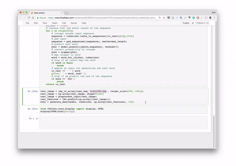
# Load and image, preprocess it for IR2, extract features and generate the HTML
test_image = img_to_array(load_img('images/87.jpg', target_size=(299, 299)))
test_image = np.array(test_image, dtype=float)
test_image = preprocess_input(test_image)
test_features = IR2.predict(np.array([test_image]))
generate_desc(model, tokenizer, np.array(test_features), 100)
输出

生成好的页面
如果你点击上面的链接后看不到内容,那么需要右击选择 “显示网页源代码”。这是对应的 原始网站。
我犯的错误
- 在我的认知里 LSTMs 比 CNNs 更重。 当我展开所有的 LSTMs,它们变得更容易理解。Fast.ai’s video on RNNs 里写的很棒。另外,不要尝试去了解它们怎样工作,专注于输入和输出功能就好了。
- 着手构建一个词汇表比弄一个巨大的词汇库简单多了。 这也适用于字体、div 尺寸、hex colors 、变量名和普通的单词。
- 大部分库都是用来解析文本文档而非代码的。 在文档里,一切东西都以空格分隔,但是在代码里,你需要定制解析。
- 可以使用在 Imagenet 训练好的模型来提取特性。 由于 Imagenet 里只有少量的 web 图片所以这可能有悖于常理。虽然和由 scratch 训练的 pix2code 模型相比错误率高达 30% ,但使用基于 web 截图的由 inception-resnet 训练的模型是一件很有趣的事。
Bootstrap 版本
在最终版本里,使用 pix2code paper 上面生成好的 bootstrap 网站数据集。通过引入 Twitter 的 bootstrap, 可以合并 HTML 和 CSS,减少词汇的体积。
我们将要为之前没有见过的截图生成标记。我们还会深入关于怎样将截图转换成代码的知识。
我们将使用 17 个简化的 tokens 来转换成 HTML 和 CSS,而不是在 bootstrap 标签上训练。数据集包含了1500 个测试截图和 250 个符合要求的图片。每个截图平均有 65 个 tokens,共有 96925 个训练例子。
通过在 pix2code paper 里定制模型,可以预测 97% 的 web 组件 (使用 BLEU 4-ngram 贪婪搜索模式后,还会更高)。

端到端接近
在图片识别模型抽出的预训练模型效果很不错。但是经过一些尝试后,我意识到 pix2code 的端到端方式在这个问题能上表现的更出色。训练好的模型还没有在 web 数据上训练,它们需要手动来分类。
在这个模型里,我们把预训练图片特性替换成了一个轻量的卷积神经网络。我们使用了 strides 而不是 max-pooling 来提高信息密度。这样就可以获得前端元素的位置和颜色。

有两个核心模型可以做到这点:卷积神经网络 (CNN)和递归神经网络 (RNN)。最常见的递归神经网络就是 long-short term memory (LSTM),这也是我更倾向的模型。
有很多的出色的 CNN 教程,我在之前的文章里也有提到过。在这里,我将会专注于 LSTMs。
了解 LSTMs 里面的 timesteps
LSTMs 里面最难理解的就是 timesteps。BP 神经网络可以看成是两个 timesteps。 如果给出 "Hello, " 它会预测出 “World.”。但是它很难预测更多的 timesteps。在下面的例子里,输入有 4 个timesteps,每一个对应一个单词。
LSTMs 由包含 timesteps 的输入组成。它是为有序信息定制的神经网络。如果展开模型看起来像下面这样。对于每个向下的 step,具有同样的权重。用一组权重来做为前一个输出,另一组做为新的输入。

加权的输入和输出被合并添加到 activation 里。这是这个 timestep 的输出。由于我们复用了权重,它们从多个输入里重组了信息构建了新的知识系列。
下面是在 LSTM 里处理每个 timestep 的过程的简单描述:

如果想更好的理解这一逻辑,我建议通过 Andrew Trask 的教程 来亲自用 scratch 构建一个 RNN。
了解 LSTM 层里面的单元
每个 LSTM 层里面的单元数量决定了存储的能力。这也反应了每个输出特性的大小。再次,特性是一个用来在不同层之间传输信息的长列表的数字。
LSTM 层里的单元跟踪学习不同的语句。下面是一个单元跟踪 row div 信息的可视化表述。这是一个简化过了的训练 bootstrap 模型的代码。

每个 LSTM 单元维护了一个 cell 的状态。可以把 cell 状态理解为内存。权重和 activations 用不同的方式修改状态。这可以让 LSTM 层在信息保持和丢弃的时候更好的契合。
除了给每个输入传入一个输出特性,还可以转发 cell 状态,cell 状态就是 LSTM 里每个单元的一个值。如果需要了解更多 LSTM 组件的交互,建议参考 Golah 的教程,Jayasiri 的 Nummpy 实现,以及 [Karphay 的讲座](Karphay’s lecture)和资料。
dir_name = 'resources/eval_light/'
# Read a file and return a string
def load_doc(filename):
    file = open(filename, 'r')
    text = file.read()
    file.close()
    return text
def load_data(data_dir):
    text = []
    images = []
    # Load all the files and order them
    all_filenames = listdir(data_dir)
    all_filenames.sort()
    for filename in (all_filenames):
        if filename[-3:] == "npz":
            # Load the images already prepared in arrays
            image = np.load(data_dir+filename)
            images.append(image['features'])
        else:
            # Load the boostrap tokens and rap them in a start and end tag
            syntax = '<START> ' + load_doc(data_dir+filename) + ' <END>'
            # Seperate all the words with a single space
            syntax = ' '.join(syntax.split())
            # Add a space after each comma
            syntax = syntax.replace(',', ' ,')
            text.append(syntax)
    images = np.array(images, dtype=float)
    return images, text
train_features, texts = load_data(dir_name)
# Initialize the function to create the vocabulary
tokenizer = Tokenizer(filters='', split=" ", lower=False)
# Create the vocabulary
tokenizer.fit_on_texts([load_doc('bootstrap.vocab')])
# Add one spot for the empty word in the vocabulary
vocab_size = len(tokenizer.word_index) + 1
# Map the input sentences into the vocabulary indexes
train_sequences = tokenizer.texts_to_sequences(texts)
# The longest set of boostrap tokens
max_sequence = max(len(s) for s in train_sequences)
# Specify how many tokens to have in each input sentence
max_length = 48
def preprocess_data(sequences, features):
    X, y, image_data = list(), list(), list()
    for img_no, seq in enumerate(sequences):
        for i in range(1, len(seq)):
            # Add the sentence until the current count(i) and add the current count to the output
            in_seq, out_seq = seq[:i], seq[i]
            # Pad all the input token sentences to max_sequence
            in_seq = pad_sequences([in_seq], maxlen=max_sequence)[0]
            # Turn the output into one-hot encoding
            out_seq = to_categorical([out_seq], num_classes=vocab_size)[0]
            # Add the corresponding image to the boostrap token file
            image_data.append(features[img_no])
            # Cap the input sentence to 48 tokens and add it
            X.append(in_seq[-48:])
            y.append(out_seq)
    return np.array(X), np.array(y), np.array(image_data)
X, y, image_data = preprocess_data(train_sequences, train_features)
#Create the encoder
image_model = Sequential()
image_model.add(Conv2D(16, (3, 3), padding='valid', activation='relu', input_shape=(256, 256, 3,)))
image_model.add(Conv2D(16, (3,3), activation='relu', padding='same', strides=2))
image_model.add(Conv2D(32, (3,3), activation='relu', padding='same'))
image_model.add(Conv2D(32, (3,3), activation='relu', padding='same', strides=2))
image_model.add(Conv2D(64, (3,3), activation='relu', padding='same'))
image_model.add(Conv2D(64, (3,3), activation='relu', padding='same', strides=2))
image_model.add(Conv2D(128, (3,3), activation='relu', padding='same'))
image_model.add(Flatten())
image_model.add(Dense(1024, activation='relu'))
image_model.add(Dropout(0.3))
image_model.add(Dense(1024, activation='relu'))
image_model.add(Dropout(0.3))
image_model.add(RepeatVector(max_length))
visual_input = Input(shape=(256, 256, 3,))
encoded_image = image_model(visual_input)
language_input = Input(shape=(max_length,))
language_model = Embedding(vocab_size, 50, input_length=max_length, mask_zero=True)(language_input)
language_model = LSTM(128, return_sequences=True)(language_model)
language_model = LSTM(128, return_sequences=True)(language_model)
#Create the decoder
decoder = concatenate([encoded_image, language_model])
decoder = LSTM(512, return_sequences=True)(decoder)
decoder = LSTM(512, return_sequences=False)(decoder)
decoder = Dense(vocab_size, activation='softmax')(decoder)
# Compile the model
model = Model(inputs=[visual_input, language_input], outputs=decoder)
optimizer = RMSprop(lr=0.0001, clipvalue=1.0)
model.compile(loss='categorical_crossentropy', optimizer=optimizer)
#Save the model for every 2nd epoch
filepath="org-weights-epoch-{epoch:04d}--val_loss-{val_loss:.4f}--loss-{loss:.4f}.hdf5"
checkpoint = ModelCheckpoint(filepath, monitor='val_loss', verbose=1, save_weights_only=True, period=2)
callbacks_list = [checkpoint]
# Train the model
model.fit([image_data, X], y, batch_size=64, shuffle=False, validation_split=0.1, callbacks=callbacks_list, verbose=1, epochs=50)
精确测试
找到合适的方式测量准确性很难。你可能会说可以一个单词一个单词对比呀。如果一个单词一个单词对比,可能会是 0% 的准确率。但是如果移动一个单词,可能准确率就变成了 99%。
我使用的是 BLEU 记分制,它是机器翻译和图片识别领域的最佳方案。它把句子拆成 4 个 n-gram,从 1-4 的单词系列。在下面预测的 “cat” 应该是 “code”。

为了获得最终分数,把每个分数乘以 25%,(4/5) * 0.25 + (2/4) * 0.25 + (1/3) * 0.25 + (0/2) * 0.25 = 0.2 + 0.125 + 0.083 + 0 = 0.408 。总分在乘以句子长度误差。由于在我们的例子里长度是正确的,可以忽略。
还可以增大 n-grams 的数目来让它更难。四个 n-gram 模型是人工翻译最好的测试模型。我建议用下面的代码多运行一些测试或者读一读它的文档。
#Create a function to read a file and return its content
def load_doc(filename):
    file = open(filename, 'r')
    text = file.read()
    file.close()
    return text
def load_data(data_dir):
    text = []
    images = []
    files_in_folder = os.listdir(data_dir)
    files_in_folder.sort()
    for filename in tqdm(files_in_folder):
        #Add an image
        if filename[-3:] == "npz":
            image = np.load(data_dir+filename)
            images.append(image['features'])
        else:
        # Add text and wrap it in a start and end tag
            syntax = '<START> ' + load_doc(data_dir+filename) + ' <END>'
            #Seperate each word with a space
            syntax = ' '.join(syntax.split())
            #Add a space between each comma
            syntax = syntax.replace(',', ' ,')
            text.append(syntax)
    images = np.array(images, dtype=float)
    return images, text
#Intialize the function to create the vocabulary
tokenizer = Tokenizer(filters='', split=" ", lower=False)
#Create the vocabulary in a specific order
tokenizer.fit_on_texts([load_doc('bootstrap.vocab')])
dir_name = '../../../../eval/'
train_features, texts = load_data(dir_name)
#load model and weights
json_file = open('../../../../model.json', 'r')
loaded_model_json = json_file.read()
json_file.close()
loaded_model = model_from_json(loaded_model_json)
# load weights into new model
loaded_model.load_weights("../../../../weights.hdf5")
print("Loaded model from disk")
# map an integer to a word
def word_for_id(integer, tokenizer):
    for word, index in tokenizer.word_index.items():
        if index == integer:
            return word
    return None
print(word_for_id(17, tokenizer))
# generate a description for an image
def generate_desc(model, tokenizer, photo, max_length):
    photo = np.array([photo])
    # seed the generation process
    in_text = '<START> '
    # iterate over the whole length of the sequence
    print('\nPrediction---->\n\n<START> ', end='')
    for i in range(150):
        # integer encode input sequence
        sequence = tokenizer.texts_to_sequences([in_text])[0]
        # pad input
        sequence = pad_sequences([sequence], maxlen=max_length)
        # predict next word
        yhat = loaded_model.predict([photo, sequence], verbose=0)
        # convert probability to integer
        yhat = argmax(yhat)
        # map integer to word
        word = word_for_id(yhat, tokenizer)
        # stop if we cannot map the word
        if word is None:
            break
        # append as input for generating the next word
        in_text += word + ' '
        # stop if we predict the end of the sequence
        print(word + ' ', end='')
        if word == '<END>':
            break
    return in_text
max_length = 48
# evaluate the skill of the model
def evaluate_model(model, descriptions, photos, tokenizer, max_length):
    actual, predicted = list(), list()
    # step over the whole set
    for i in range(len(texts)):
        yhat = generate_desc(model, tokenizer, photos[i], max_length)
        # store actual and predicted
        print('\n\nReal---->\n\n' + texts[i])
        actual.append([texts[i].split()])
        predicted.append(yhat.split())
    # calculate BLEU score
    bleu = corpus_bleu(actual, predicted)
    return bleu, actual, predicted
bleu, actual, predicted = evaluate_model(loaded_model, texts, train_features, tokenizer, max_length)
#Compile the tokens into HTML and css
dsl_path = "compiler/assets/web-dsl-mapping.json"
compiler = Compiler(dsl_path)
compiled_website = compiler.compile(predicted[0], 'index.html')
print(compiled_website )
print(bleu)
输出

输出结果的例子的链接
我犯的错误
- 理解模型的弱点而不是测试随机的模型。 最初我使用了一个随机的模型类似于 batch normalization 和 bidirectional networks,尝试花更多精力在上面。后来查看了测试数据发现它无法准确预测颜色和位置等信息,我意识到了 CNN 在某些放面有缺陷。所以我把 mapooling 替换成了更新的 strides。validation 损失从 0.12 降到了 0.02,BLEU 分数从 85% 增加到了 97%。
- 如果有现成的就使用预训练的数据。 用一个小数据集的图片预训练模型会提高性能。根据我的经验,端到端模型训练起来很慢并且需要更多的内存,只提高了 30% 的准确性。
- 如果把你的模型运行在远程服务器上的话需要注意一些细节。 在我的 mac 上,文件按字母顺序读取。可是在服务器上读取顺序是随机的。这样截图和代码之间就不能匹配了。虽然可能有相交,但是数据比我修复这一问题后糟糕了 50%。
- 确保你了解了库的功能。 比如在你的词汇里面的空格产生的空 token。当我添加时,它并没有添加这些 tokens。在调试之后我只注意到了最终输出了多次,并没有预测出 “single” token。在排查后,我意识它甚至到不在词汇表中。因此,最好按和词汇表里相同的顺序训练测试。
- 体验的时候尽量使用轻量级的库。 使用 GRUs 而不是 LSTMs,这样每个 epoch 能减少 30% ,同时对性能又不会有太大的影响。
下一步
前端开发是深度学习的一个重要的应用场景。生成数据很容易,当前的深度学习算法能覆盖到大部分逻辑。
另一个更令人振奋的领域是 在 LSTMs 里使用 attention。这不仅能提升准确度,还能可视化。CNN 则更专注于生成代码。
Attention 是代码标签、样式、脚本和后端间沟通的桥梁。Attention 层可以打通变量,能够在不同编程语言间通讯。
在最终版本里,需要考虑下怎样用一个可扩展的方式来生成数据。接下来就可以添加字体、颜色、单词甚至是动画。
目前为止,大部分的流程都是通过 sketches 设计然后把它们转换成模板 app。在未来两年时间里,我们在纸上画一个 APP,前端会在 1 秒内得到页面。现在 Airbnb 的设计团队和 Uizard 已经有了两个原型。
这里是更多的玩法。
玩法
起步
- 运行所有的方法
- 尝试不同的 hyper 参数
- 测试不同的 LSTM 模型
- 使用不同的数据集实现模型。(可以通过
--data emilwallner/datasets/100k-html:dataflag 方便的在 FloydHub 上挂载这一工具集)
更多玩法
- 创建一个固定的随机的 app/web 自动代码生成器。
- sketch 的 app model 数据。自动转换 app/web 截图到 sketches,使用 GAN 来创建分类。
- 应用 attention 层来可视化每个预测焦的预测,类似于这个模型。
- 创建一个模块化功能的框架。已经有了字体、颜色、布局的编码模块,把它们组合成一个解码器。建议从实现图像特性开始。
- 为机器提供简单的 HTML 组件,教会它使用 CSS 生成动画。采用 attention 方法专注于两个输入源一定很有趣。
原文链接:How you can train an AI to convert your design mockups into HTML and CSS,作者:Emil Wallner